DATA WAREHOUSE DESIGN APPROACHES

Data warehouse design is one of the key technique in building the data warehouse. Choosing a right data warehouse design can save the project time and cost. Basically there are two data warehouse design approaches are popular.

Bottom-Up Design:

In the bottom-up design approach, the data marts are created first to provide reporting capability. A data mart addresses a single business area such as sales, Finance etc. These data marts are then integrated to build a complete data warehouse.  The integration of data marts is implemented using data warehouse bus architecture. In the bus architecture, a dimension is shared between facts in two or more data marts. These dimensions are called conformed dimensions. These conformed dimensions are integrated from data marts and then data warehouse is built.

Advantages of bottom-up design are:

• This model contains consistent data marts and these data marts can be delivered quickly.

• As the data marts are created first, reports can be generated quickly.

• The data warehouse can be extended easily to accommodate new business units. It is just creating new data marts and then integrating with other data marts.

Disadvantages of bottom-up design are:

• The positions of the data warehouse and the data marts are reversed in the bottom-up approach design.

Top-Down Design:

In the top-down design approach the, data warehouse is built first. The data marts are then created from the data warehouse.

Advantages of top-down design are:

• Provides consistent dimensional views of data across data marts, as all data marts are loaded from the data warehouse.
• This approach is robust against business changes. Creating a new data mart from the data warehouse is very easy.

Disadvantages of top-down design are:

• This methodology is inflexible to changing departmental needs during implementation phase.
• It represents a very large project and the cost of implementing the project is significant.

TYPES OF DIMENSIONS IN DATA WAREHOUSE

A dimension table consists of the attributes about the facts. Dimensions store the textual descriptions of the business. With out the dimensions, we cannot measure the facts. The different types of dimension tables are explained in detail below.

Conformed Dimension:

Conformed dimensions mean the exact same thing with every possible fact table to which they are joined.

Eg: The date dimension table connected to the sales facts is identical to the date dimension connected to the inventory facts.

Junk Dimension:

A junk dimension is a collection of random transactional codes flags and/or text attributes that are unrelated to any particular dimension. The junk dimension is simply a structure that provides a convenient place to store the junk attributes.

Eg: Assume that we have a gender dimension and marital status dimension. In the fact table we need to maintain two keys referring to these dimensions. Instead of that create a junk dimension which has all the combinations of gender and marital status (cross join gender and marital status table and create a junk table). Now we can maintain only one key in the fact table.

Degenerated Dimension:

A degenerate dimension is a dimension which is derived from the fact table and doesn't have its own dimension table.

Eg: A transactional code in a fact table.

Role-playing dimension:

Dimensions which are often used for multiple purposes within the same database are called role-playing dimensions. For example, a date dimension can be used for “date of sale", as well as "date of delivery", or "date of hire". 

Conformed Dimension

A conformed dimension is a dimension that has exactly the same meaning and content when being referred from different fact tables. A conformed dimension can refer to multiple tables in multiple data marts within the same organization. For two dimension tables to be considered as conformed, they must either be identical or one must be a subset of another. There cannot be any other type of difference between the two tables. For example, two dimension tables that are exactly the same except for the primary key are not considered conformed dimensions.

Why is conformed dimension important? This goes back to the definition of data warehouse being "integrated." Integrated means that even if a particular entity had different meanings and different attributes in the source systems, there must be a single version of this entity once the data flows into the data warehouse.

The time dimension is a common conformed dimension in an organization. Usually the only rule to consider with the time dimension is whether there is a fiscal year in addition to the calendar year and the definition of a week. Fortunately, both are relatively easy to resolve. In the case of fiscal vs. calendar year, one may go with either fiscal or calendar, or an alternative is to have two separate conformed dimensions, one for fiscal year and one for calendar year. The definition of a week is also something that can be different in large organizations: Finance may use Saturday to Friday, while marketing may use Sunday to Saturday. In this case, we should decide on a definition and move on. The nice thing about the time dimension is once these rules are set, the values in the dimension table will never change. For example, October 16th will never become the 15th day in October.

Not all conformed dimensions are as easy to produce as the time dimension. An example is the customer dimension. In any organization with some history, there is a high likelihood that different customer databases exist in different parts of the organization. To achieve a conformed customer dimension means those data must be compared against each other, rules must be set, and data must be cleansed. In addition, when we are doing incremental data loads into the data warehouse, we'll need to apply the same rules to the new values to make sure we are only adding truly new customers to the customer dimension.

Building a conformed dimension also part of the process in master data management, or MDM. In MDM, one must not only make sure the master data dimensions are conformed, but that conformity needs to be brought back to the source systems. 

Junk Dimension

In data warehouse design, frequently we run into a situation where there are yes/no indicator fields in the source system. Through business analysis, we know it is necessary to keep such information in the fact table. However, if keep all those indicator fields in the fact table, not only do we need to build many small dimension tables, but the amount of information stored in the fact table also increases tremendously, leading to possible performance and management issues.

Junk dimension is the way to solve this problem. In a junk dimension, we combine these indicator fields into a single dimension. This way, we'll only need to build a single dimension table, and the number of fields in the fact table, as well as the size of the fact table, can be decreased. The content in the junk dimension table is the combination of all possible values of the individual indicator fields.

Let's look at an example. Assuming that we have the following fact table:

In this example, the last 3 fields are all indicator fields. In this existing format, each one of them is a dimension. Using the junk dimension principle, we can combine them into a single junk dimension, resulting in the following fact table:

Note that now the number of dimensions in the fact table went from 7 to 5.

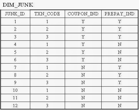
The content of the junk dimension table would look like the following:

In this case, we have 3 possible values for the TXN_CODE field, 2 possible values for the COUPON_IND field, and 2 possible values for the PREPAY_IND field. This results in a total of 3 x 2 x 2 = 12 rows for the junk dimension table.

By using a junk dimension to replace the 3 indicator fields, we have decreased the number of dimensions by 2 and also decreased the number of fields in the fact table by 2. This will result in a data warehousing environment that offer better performance as well as being easier to manage.

Data Modeling - Conceptual, Logical, And Physical Data Models

·   Data Modeling - Conceptual, Logical, And Physical Data Models

·   

    The three levels of data modeling, conceptual data model, logical data model, and physical data model, were discussed in prior sections. Here we compare these three types of data models. The table below compares the different features:

Feature	Conceptual	Logical	Physical
Entity Names	✓	✓
Entity Relationships	✓	✓
Attributes		✓
Primary Keys		✓	✓
Foreign Keys		✓	✓
Table Names			✓
Column Names			✓
Column Data Types			✓

·         

·   We can see that the complexity increases from conceptual to logical to physical. This is why we always first start with the conceptual data model (so we understand at high level what are the different entities in our data and how they relate to one another), then move on to the logical data model (so we understand the details of our data without worrying about how they will actually implemented), and finally the physical data model (so we know exactly how to implement our data model in the database of choice). In a data warehousing project, sometimes the conceptual data model and the logical data model are considered as a single deliverable. 

Physical Data Model

Physical data model represents how the model will be built in the database. A physical database model shows all table structures, including column name, column data type, column constraints, primary key, foreign key, and relationships between tables. Features of a physical data model include:

• Specification all tables and columns.
• Foreign keys are used to identify relationships between tables.
• Denormalization may occur based on user requirements.
• Physical considerations may cause the physical data model to be quite different from the logical data model.
• Physical data model will be different for different RDBMS. For example, data type for a column may be different between MySQL and SQL Server.

The steps for physical data model design are as follows:

1. Convert entities into tables.
2. Convert relationships into foreign keys.
3. Convert attributes into columns.
4. Modify the physical data model based on physical constraints / requirements.

The figure below is an example of a physical data model.

Physical Data Model

Comparing the logical data model shown above with the logical data model diagram, we see the main differences between the two:

• Entity names are now table names.
• Attributes are now column names.
• Data type for each column is specified. Data types can be different depending on the actual database being used. 

Logical Data Model

A logical data model describes the data in as much detail as possible, without regard to how they will be physical implemented in the database. Features of a logical data model include:

• Includes all entities and relationships among them.
• All attributes for each entity are specified.
• The primary key for each entity is specified.
• Foreign keys (keys identifying the relationship between different entities) are specified.
• Normalization occurs at this level.

The steps for designing the logical data model are as follows:

1. Specify primary keys for all entities.
2. Find the relationships between different entities.
3. Find all attributes for each entity.
4. Resolve many-to-many relationships.
5. Normalization.

The figure below is an example of a logical data model.

Logical Data Model

Comparing the logical data model shown above with the conceptual data model diagram, we see the main differences between the two:

• In a logical data model, primary keys are present, whereas in a conceptual data model, no primary key is present.
• In a logical data model, all attributes are specified within an entity. No attributes are specified in a conceptual data model.
• Relationships between entities are specified using primary keys and foreign keys in a logical data model. In a conceptual data model, the relationships are simply stated, not specified, so we simply know that two entities are related, but we do not specify what attributes are used for this relationship. 

Conceptual Data Model

A conceptual data model identifies the highest-level relationships between the different entities. Features of conceptual data model include:

• Includes the important entities and the relationships among them.
• No attribute is specified.
• No primary key is specified.

The figure below is an example of a conceptual data model.

Conceptual Data Model

From the figure above, we can see that the only information shown via the conceptual data model is the entities that describe the data and the relationships between those entities. No other information is shown through the conceptual data model.