Join tables using different DB Sources

One of the advantages of BI EE is its ability to make cross database joins. Currently, BI Server component of BI EE supports database joins across any database. This feature is primarily meant for joins between a database and some lookup tables coming from Excel files. Though this would work for databases too, its not recommended to use them in a production environment since BI EE does the joins in memory by extracting the data from the source databases first. We will see how to go about creating a simple cross database join today. There is not much difference in the way we actually set up the repository. But still i thought this deserves its own blog entry since its a very unique feature of BI EE. We shall simulate this using 2 simple tables. One table (EMP table of the normal Oracle SCOTT schema) would be from Oracle and the other table would be from an Excel file. For demonstration purposes we shall be exporting the normal DEPT table from the SCOTT schema in the form of an excel file. So, basically we have 2 tables.
EMP Table in an Oracle Database
DEPT Table in an EXCEL file
Our final aim is to create a simple report in Answers with data 
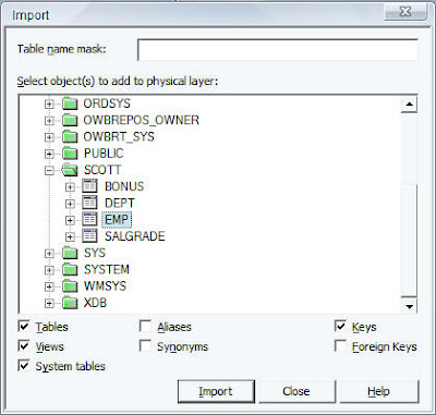
coming in from both the EMP table and the DEPT table. In order to do that the first step is to import the EMP Table from the Oracle Database into the repository.
      
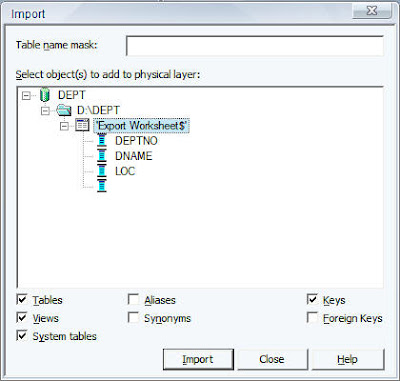
Similarly, import the Excel file (which is basically an export of the DEPT table) using ODBC.
      
      
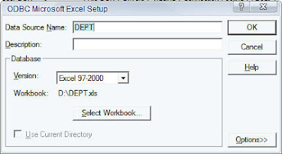
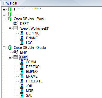
So, our repository should basically have 2 tables in 2 different databases as shown below.
      
Once this is done, the next step is to create a join between these 2 tables in the physical layer.Typically, if you go to the physical layer diagram, it would allow joins only between tables in the same database. 
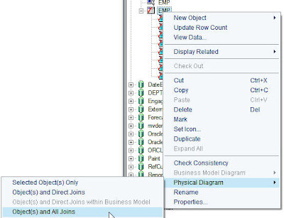
In order to achieve cross-database joins, the first step is to right click on the EMP table and then click on Physical Diagram -> All Objects and Joins.
      
In the same way (ensure that the physical Diagram window is open), right click and click on view physical diagram on the DEPT Excel table source. That will automatically bring both the tables inside the physical layer.
      
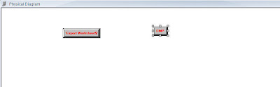
Now, create a database join between both the tables using DEPTNO as the join column.
      
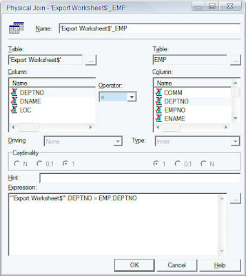
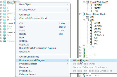
Once this is done, save the changes made in the repository. Now, create a new Business Model Cross DB join. Drag and drop both the tables (DEPT and EMP) from the physical layer into the Cross DB join Business Model. Then right click on Cross DB Join and click on view the Business Model diagram.
      
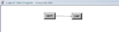
Similar to what we did in the Physical layer, create a foreign key join between DEPT and the EMP table based on DEPTNO column.
      
Once this is done, drag and drop the Business Model into the Presentation layer and save the repository. Ensure that your repository is clear of any warnings or errors. Once this is done, go to Answers and try creating a simple report having DNAME and SAL as thecolumns.
      
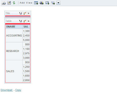
As you see, we have now created a report that contains data from 2 different data sources. The BI Server does the joins in the background. 
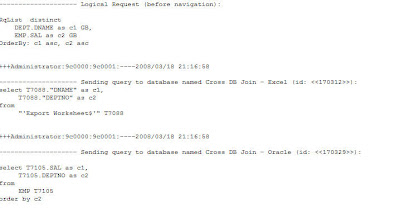
To see what exactly the BI Server, is doing, lets look at the logs to get the exact SQL. You would basically see 2 SQLs. They are
select T7105.SAL as c1,
T7105.DEPTNO as c2
from
EMP T7105
order by c2
and
select T7088.”DNAME” as c1,
T7088.”DEPTNO” as c2
from
“‘Export Worksheet$'” T7088
      

Creating new user (using SQL Plus)

Creating new user (using SQL Plus)
Basic SQL Plus commands:
- connect: connects to a database - disconnect: logs off but does not exit - exit: exists
Open SQL Plus and log:
/ as sysdba
The sysdba is a role and is like "root" on unix or "Administrator" on Windows. It sees all, can do all. Internally, if you connect as sysdba, your schema name will appear to be SYS.
Create an user:
SQL> create user johny identified by 1234;
View all users and check if the user johny is there:
SQL> select username from dba_users;
If you try to login as johny now you would get an error:
ERROR: ORA-01045: user JOHNY lacks CREATE SESSION privilege; logon denied
The user to login needs at least create session priviledge so we have to grant this privileges to the user:
SQL> grant create session to johny;
Now you are able to connect as the user johny:
username: johny password: 1234
To get rid of the user you can drop it:
SQL> drop user johny;

That was basic example to show how to create an user. It might be more complex. Above we created an user who's objects are stored in the database default tablespace. To have database tidy we should place users objects to his own space (tablespace is an allocation of space in the database that can contain schema objects).
Show already created tablespaces:
SQL> select tablespace_name from dba_tablespaces;
Create tablespace:
SQL> create tablespace johny_tabspace 2 datafile 'johny_tabspace.dat' 3 size 10M autoextend on;
Create temporary tablespace (Temporaty tablespace is an allocation of space in the database that can contain transient data that persists only for the duration of a session. This transient data cannot be recovered after process or instance failure.):
SQL> create temporary tablespace johny_tabspace_temp 2 tempfile 'johny_tabspace_temp.dat' 3 size 5M autoextend on;
Create the user:
SQL> create user johny 2 identified by 1234 3 default tablespace johny_tabspace 4 temporary tablespace johny_tabspace_temp;
Grant some privileges:
SQL> grant create session to johny; SQL> grant create table to johny; SQL> grant unlimited tablespace to johny;
Login as johny and check what privileges he has:
SQL> select * from session_privs; PRIVILEGE ---------------------------------------- CREATE SESSION UNLIMITED TABLESPACE CREATE TABLE
With create table privilege the user can create tables:
SQL> create table johny_table 2 ( 3 id int not null, 4 text varchar2(1000), 5 primary key (id) 6 );
Insert data:
SQL> insert into johny_table (id, text) 2 values (1, 'This is some text.');
Select:
SQL> select * from johny_table; ID TEXT -------------------------- 1 This is some text.
To get DDL data you can use DBMS_METADATA package that "provides a way for you to retrieve metadata from the database dictionary as XML or creation DDL and to submit the XML to re-create the object.". 
For table:
SQL> set pagesize 0 SQL> set long 90000 SQL> set feedback off SQL> set echo off SQL> SELECT DBMS_METADATA.GET_DDL('TABLE',u.table_name) FROM USER_TABLES u;
Result:
CREATE TABLE "JOHNY"."JOHNY_TABLE" ( "ID" NUMBER(*,0) NOT NULL ENABLE, "TEXT" VARCHAR2(1000), PRIMARY KEY ("ID") USING INDEX PCTFREE 10 INITRANS 2 MAXTRANS 255 STORAGE(INITIAL 65536 NEXT 1048576 MINEXTENTS 1 MAXEXTENTS 2147483645 PCTINCREASE 0 FREELISTS 1 FREELIST GROUPS 1 BUFFER_POOL DEFAULT FLASH_CACHE DE FAULT CELL_FLASH_CACHE DEFAULT) TABLESPACE "JOHNY_TABSPACE" ENABLE ) SEGMENT CREATION IMMEDIATE PCTFREE 10 PCTUSED 40 INITRANS 1 MAXTRANS 255 NOCOMPRESS LOGGING STORAGE(INITIAL 65536 NEXT 1048576 MINEXTENTS 1 MAXEXTENTS 2147483645 PCTINCREASE 0 FREELISTS 1 FREELIST GROUPS 1 BUFFER_POOL DEFAULT FLASH_CACHE DE FAULT CELL_FLASH_CACHE DEFAULT) TABLESPACE "JOHNY_TABSPACE"
For index:
SQL> set pagesize 0 SQL> set long 90000 SQL> set feedback off SQL> set echo off SQL> SELECT DBMS_METADATA.GET_DDL('INDEX',u.index_name) FROM USER_INDEXES u;
Result:
CREATE UNIQUE INDEX "JOHNY"."SYS_C0013353" ON "JOHNY"."JOHNY_TABLE" ("ID") PCTFREE 10 INITRANS 2 MAXTRANS 255 STORAGE(INITIAL 65536 NEXT 1048576 MINEXTENTS 1 MAXEXTENTS 2147483645 PCTINCREASE 0 FREELISTS 1 FREELIST GROUPS 1 BUFFER_POOL DEFAULT FLASH_CACHE DE FAULT CELL_FLASH_CACHE DEFAULT) TABLESPACE "JOHNY_TABSPACE"

Custom Date format in the Dashboard Prompts IN OBIEE

Change the Custom Date format in the Dashboard Prompts

How to Set default My Account -> User ->Performance : Locale , Time Zone and Language and Analytics’s Calendar default Date format

  1. To set default User -> Preference -> location modify the
    <MIDDLEWARE_HOME>/Oracle_BI1/bifoundation/web/display/localemappings.xml
    Replace
    <when matches=”en*”><localeDefinition name=”en-us”/></when>    With
   <when matches=”en*”><localeDefinition name=”en-au”/></when>
  1. To set the Time Zone  and Data Time Zone Offset , add the following entries in instanceconfig.xml
    <TimeZone>

         <DefaultDataOffset>600</DefaultDataOffset>

         <Logging>(GMT+10:00) Canberra, Melbourne, Sydney</Logging>

         <DefaultUserPreferred>(GMT+10:00) Canberra, Melbourne, Sydney</DefaultUserPreferred>

         <DefaultDataDisplay>(GMT+10:00) Canberra, Melbourne, Sydney</DefaultDataDisplay>

    </TimeZone>

    For more details:  Oracle® Fusion Middleware System Administrator’s Guide for Oracle Business Intelligence Enterprise Edition 11g Release 1 (11.1.1) -15 Configuring Time Zones
  2. To restrict the location and language for account  (Drop down list of location and language) add entries in instanceconfig.xml :
    <Localization>

    <AllowedLanguages>en</AllowedLanguages>
    <AllowedLocales>en-au</AllowedLocales>
    </Localization>
  3. To set Default calendar Date formatting
    <MIDDLEWARE_HOME>/Oracle_BI1/bifoundation/web/display/localedefinitions.xml :
    Replace below properties with appropriate value
    <property name=”dateShortFormat”>d/MM/yyyy</property>

    <property name=”dateOrder”>dmy</property>

Why OBIEE 11G is preferrable?

OBIEE 11g is more preferable than OBIEE 10g as it has got remarkable features which are as follows:

Multiple Subject Areas:
In this release, you can work with multiple subject areas. In addition to the primary subject area that you select when you create a new analysis, filter, or dashboard prompt, you can include additional subject areas that are related to the primary subject area with which to work.
Interaction with Other Oracle Products: - Oracle BI Publisher is a fully integrated member of the Oracle BI EE suite by default.
– Oracle Hyperion Smart View is available for download from the Oracle BI EE Home page.
– The integration of Oracle BI EE with Oracle Business Intelligence Add-in for Microsoft Office has been enhanced.

Enhanced Drill-down Functionality:
In this release, the drill-down functionality is been modified so that one can drill-in place and see the impact without effecting the other values of the same attribute.
eg:  The drill-down functionality is been applied on a column(say ‘Year’).
If the end-user selects any value (say ‘2010’), the drill-in place occurs on that column and shows the child level attributes for that particular value without effecting the report structure wherein the remaining values of the same column are undisturbed.
Web Catalog Migration:
Another easier, more attractive approach is to abandon the file system copy altogether and use the Catalog Manager to facilitate the movement of only the shared folder, or some portion of it, from Dev to Prod. A new enhancement in 11g is the ability to do web catalog Archive and Unarchive operations from within Answers.
Authorization:
Authorization in 10g was achieved using a combination of Users, Groups and association of privileges and object permissions to users and Groups. Two keys changes to Authorization in OBIEE 11g are:
  1. Application Roles
  2. Policies / Permission Groups
Application Roles are introduced in OBIEE 11g. An application role is specific to the application. They can be mapped to other application roles defined in the same application scope and also to enterprise users or groups, and they are used in authorization decisions. Application roles in 11g take the place of Groups in 10g within OBIEE application. In OBIEE 10g, any changes to corporate LDAP groups require a corresponding change to Groups and their permission assignment. In OBIEE 11g, Application roles provide insulation between permission definitions and corporate LDAP Groups. Permissions are defined at Application Role level and changes to LDAP groups just require a reassignment of the Group to the Application Roles.
Permissions and privileges are assigned to Application Roles and users in OBIEE 11g compared to Groups and Users in 10g.
Application policies are the authorization policies that an application relies upon for controlling access to its resources. An Application Role is defined by the Application Policy.
In OBIEE 10g, the permission to manage repositories and Impersonation were assigned to “Administrators” group with no control to separate these permissions in the Administrators group. Hence user “Administrator” also had the permission to impersonate. In OBI11g, BIAdministrator does not have the permission to impersonate. This gives more flexibility to have multiple users perform different administrative functions.
New Column Type and Related Operations: In this release, new column type Hierarchical Column is introduced.
Hierarchical Column holds data values that are organized and support the following hierarchy kinds:
– Level-based hierarchy,
– Parent-child hierarchy,
– Ragged or unbalanced hierarchy (in which all the lowest-level members do not have the same depth),
– Skip-level hierarchy (in which certain members do not have values for certain higher levels).

Enhancements to Views: Several of the view types have been enhanced, including:
– New Table and pivot table functionality, hierarchical columns and drag and drop columns.
– New Slider functionality on graphs and gauges views.
– New Map view type to presents data in spatial form.
– New Master-detail linking of views, which enable to establish a relationship between two or more views such that one view, called the master view, will drive data changes in one or more other views, called detail views.


SQL Functions for Time Series Calculations
PERIODROLLING is a new function that computes the sum of a measure over the period starting x units of time and ending y units of time from the current time.
AGGREGATE AT is a new function that aggregates columns based on the level or levels specified
AGO is a time series aggregation function that calculates the aggregated value from the current time back to a specified time period. In this release, the time_level argument is optional, and there are additional syntax changes.
TODATE is a time series aggregation function that aggregates a measure attribute from the beginning of a specified time period to the currently displayed time. The syntax for this function has changed in this release.

Embedded Database Functions: New supported functions EVALUATE, EVALUATE_AGGR, and EVALUATE_PREDICATE can be directly calling database functions from either Oracle Business Intelligence, or by using a Logical column (in the Logical Table source) within the metadata repository.
Key Performance Indicators (KPIs): In this release, you can create KPIs to represent business measures or metrics that you want to monitor, improve, and use to evaluate the performance of the objectives and initiatives that comprise levels of organizational strategy.
KPIs have measurable values that usually vary with time, have targets to determine a score and performance status include dimensions to allow for more specific analysis, and can be compared over time for trending purposes and to identify performance patterns.
Oracle Scorecard and Strategy Management: In this release, you can use Oracle Scorecard and Strategy Management to articulate, evaluate (scorecard), and evolve the performance of your organization or key business areas. You can use Oracle Scorecard and Strategy Management to define, depict, and monitor the progress of the strategic goals and requirements (objectives) key to corporate functions, and the tasks and projects (initiatives) that are required to achieve those goals. Oracle Scorecard and Strategy Management also enables you to either align your objectives and initiatives with traditional balanced scorecard perspectives, or to create your own to reflect your fundamental business competencies.
OBIEE ARCHITECTURE

DATA WAREHOUSE DIMENSIONAL MODELLING (TYPES OF SCHEMAS)

There are four types of schemas are available in data warehouse. Out of which the star schema is mostly used in the data warehouse designs. The second mostly used data warehouse schema is snow flake schema. We will see about these schemas in detail.

Star Schema:


A star schema is the one in which a central fact table is sourrounded by denormalized dimensional tables. A star schema can be simple or complex. A simple star schema consists of one fact table where as a complex star schema have more than one fact table.


Snow Flake Schema:


A snow flake schema is an enhancement of star schema by adding additional dimensions. Snow flake schema are useful when there are low cardinality attributes in the dimensions.


Galaxy Schema:


Galaxy schema contains many fact tables with some common dimensions (conformed dimensions). This schema is a combination of many data marts.


Fact Constellation Schema:


The dimensions in this schema are segregated into independent dimensions based on the levels of hierarchy. For example, if geography has five levels of hierarchy like teritary, region, country, state and city; constellation schema would have five dimensions instead of one. 

DATA WAREHOUSE DESIGN APPROACHES


Data Warehouse Design Approaches

Data warehouse design is one of the key technique in building the data warehouse. Choosing a right data warehouse design can save the project time and cost. Basically there are two data warehouse design approaches are popular.

Bottom-Up Design:

In the bottom-up design approach, the data marts are created first to provide reporting capability. A data mart addresses a single business area such as sales, Finance etc. These data marts are then integrated to build a complete data warehouse.  The integration of data marts is implemented using data warehouse bus architecture. In the bus architecture, a dimension is shared between facts in two or more data marts. These dimensions are called conformed dimensions. These conformed dimensions are integrated from data marts and then data warehouse is built.

Advantages of bottom-up design are:

  • This model contains consistent data marts and these data marts can be delivered quickly.
  • As the data marts are created first, reports can be generated quickly.
  • The data warehouse can be extended easily to accommodate new business units. It is just creating new data marts and then integrating with other data marts.


Disadvantages of bottom-up design are:

  • The positions of the data warehouse and the data marts are reversed in the bottom-up approach design.


Top-Down Design:

In the top-down design approach the, data warehouse is built first. The data marts are then created from the data warehouse.

Advantages of top-down design are:

  • Provides consistent dimensional views of data across data marts, as all data marts are loaded from the data warehouse.
  • This approach is robust against business changes. Creating a new data mart from the data warehouse is very easy.


Disadvantages of top-down design are:

  • This methodology is inflexible to changing departmental needs during implementation phase.
  • It represents a very large project and the cost of implementing the project is significant.

TYPES OF DIMENSIONS IN DATA WAREHOUSE

A dimension table consists of the attributes about the facts. Dimensions store the textual descriptions of the business. With out the dimensions, we cannot measure the facts. The different types of dimension tables are explained in detail below.


Conformed Dimension:

Conformed dimensions mean the exact same thing with every possible fact table to which they are joined.

Eg: The date dimension table connected to the sales facts is identical to the date dimension connected to the inventory facts.

Junk Dimension:

A junk dimension is a collection of random transactional codes flags and/or text attributes that are unrelated to any particular dimension. The junk dimension is simply a structure that provides a convenient place to store the junk attributes.

Eg: Assume that we have a gender dimension and marital status dimension. In the fact table we need to maintain two keys referring to these dimensions. Instead of that create a junk dimension which has all the combinations of gender and marital status (cross join gender and marital status table and create a junk table). Now we can maintain only one key in the fact table.

Degenerated Dimension:

A degenerate dimension is a dimension which is derived from the fact table and doesn't have its own dimension table.

Eg: A transactional code in a fact table.

Role-playing dimension:

Dimensions which are often used for multiple purposes within the same database are called role-playing dimensions. For example, a date dimension can be used for “date of sale", as well as "date of delivery", or "date of hire". 

Conformed Dimension

A conformed dimension is a dimension that has exactly the same meaning and content when being referred from different fact tables. A conformed dimension can refer to multiple tables in multiple data marts within the same organization. For two dimension tables to be considered as conformed, they must either be identical or one must be a subset of another. There cannot be any other type of difference between the two tables. For example, two dimension tables that are exactly the same except for the primary key are not considered conformed dimensions.

Why is conformed dimension important? This goes back to the definition of data warehouse being "integrated." Integrated means that even if a particular entity had different meanings and different attributes in the source systems, there must be a single version of this entity once the data flows into the data warehouse.

The time dimension is a common conformed dimension in an organization. Usually the only rule to consider with the time dimension is whether there is a fiscal year in addition to the calendar year and the definition of a week. Fortunately, both are relatively easy to resolve. In the case of fiscal vs. calendar year, one may go with either fiscal or calendar, or an alternative is to have two separate conformed dimensions, one for fiscal year and one for calendar year. The definition of a week is also something that can be different in large organizations: Finance may use Saturday to Friday, while marketing may use Sunday to Saturday. In this case, we should decide on a definition and move on. The nice thing about the time dimension is once these rules are set, the values in the dimension table will never change. For example, October 16th will never become the 15th day in October.

Not all conformed dimensions are as easy to produce as the time dimension. An example is the customer dimension. In any organization with some history, there is a high likelihood that different customer databases exist in different parts of the organization. To achieve a conformed customer dimension means those data must be compared against each other, rules must be set, and data must be cleansed. In addition, when we are doing incremental data loads into the data warehouse, we'll need to apply the same rules to the new values to make sure we are only adding truly new customers to the customer dimension.

Building a conformed dimension also part of the process in master data management, or MDM. In MDM, one must not only make sure the master data dimensions are conformed, but that conformity needs to be brought back to the source systems. 

Junk Dimension

In data warehouse design, frequently we run into a situation where there are yes/no indicator fields in the source system. Through business analysis, we know it is necessary to keep such information in the fact table. However, if keep all those indicator fields in the fact table, not only do we need to build many small dimension tables, but the amount of information stored in the fact table also increases tremendously, leading to possible performance and management issues.

Junk dimension is the way to solve this problem. In a junk dimension, we combine these indicator fields into a single dimension. This way, we'll only need to build a single dimension table, and the number of fields in the fact table, as well as the size of the fact table, can be decreased. The content in the junk dimension table is the combination of all possible values of the individual indicator fields.

Let's look at an example. Assuming that we have the following fact table:


In this example, the last 3 fields are all indicator fields. In this existing format, each one of them is a dimension. Using the junk dimension principle, we can combine them into a single junk dimension, resulting in the following fact table:

Note that now the number of dimensions in the fact table went from 7 to 5.

The content of the junk dimension table would look like the following:

In this case, we have 3 possible values for the TXN_CODE field, 2 possible values for the COUPON_IND field, and 2 possible values for the PREPAY_IND field. This results in a total of 3 x 2 x 2 = 12 rows for the junk dimension table.

By using a junk dimension to replace the 3 indicator fields, we have decreased the number of dimensions by 2 and also decreased the number of fields in the fact table by 2. This will result in a data warehousing environment that offer better performance as well as being easier to manage.

Data Modeling - Conceptual, Logical, And Physical Data Models

·   Data Modeling - Conceptual, Logical, And Physical Data Models
·   
    The three levels of data modeling, conceptual data model, logical data model, and physical data model, were discussed in prior sections. Here we compare these three types of data models. The table below compares the different features:

Feature
Conceptual
Logical
Physical
Entity Names
 
Entity Relationships
 
Attributes
 
 
Primary Keys
 
Foreign Keys
 
Table Names
 
 
Column Names
 
 
Column Data Types
 
 
·         

·   We can see that the complexity increases from conceptual to logical to physical. This is why we always first start with the conceptual data model (so we understand at high level what are the different entities in our data and how they relate to one another), then move on to the logical data model (so we understand the details of our data without worrying about how they will actually implemented), and finally the physical data model (so we know exactly how to implement our data model in the database of choice). In a data warehousing project, sometimes the conceptual data model and the logical data model are considered as a single deliverable.